

The mathematical model of the exhaust manifold has been developed following a F&E approach. Temperature and pressure are obtained from the equations of conservation of mass and energy applied to the manifold considered as a 0D volume. Estimating heat flow through manifold walls as suggested in Guzzella and Onder (2010), energy conservation equation for exhaust gases inside the manifold can be written as follows:
where Q˙in is the heat flux from the gas mixture to the manifold walls. Enthalpy of gases leaving the manifold htur and hEGR are calculated assuming that gas temperatures are equal to that inside the manifold.
In the presented model the thermal inertia of the exhaust manifold has been considered assuming a defined overall mass mw and a constant specific heat cw for the manifold walls (Figure 1). Manifold walls temperature has been assumed uniform, and its changes have bene estimated through the following differential equation:
where Q˙in and Q˙out are heat flux between gas stream and walls and between walls and ambient air, respectively. These heat fluxes can be calculated with reference to the well-known schematic description reported in Figure 1, where heat is exchanged by convection and radiation between gas flow and internal walls, by conduction through the walls and by convection and radiation between external walls and ambient air. In the proposed model, however, internal radiation has been considered negligible. Even if the real geometry of the manifold is complex, it has been modeled as a single cylindrical pipe with a proper length L to keep the calculation burden within the limits of the 0D approach.
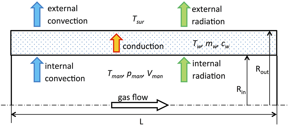 FIGURE 1. Schematic of the exhaust manifold flows.
To estimate Q˙in a specific correlation suggested in the literature for intake and exhaust systems of ICEs has been used in the following form (Depcik and Assanis, 2001):
The term Prc often assumes a value close to 1 and values for a and b are defined from measurements. The value of Nu was estimated from the Gnielinski correlation reported in Konstantinidis et al. (1997) and Kandylas and Stamatelos (1999) introducing as suggested a suitable Convective Augmentation Factor to take account of flow unsteadiness and turbulence defined as follows:
where Nueff and Nuth are effective and theoretical value respectively. The last value can be estimated through well-known correlations from Konstantinidis et al. (1997) and Kandylas and Stamatelos (1999):
and
where
and
Then convection coefficient and heat flux can be calculated, since:
and
where Pr, μ, and λ for the exhaust gas are estimated at Texh_man temperature, assumed as uniform in the exhaust manifold.
The estimation of convective heat flux from manifold walls to ambient air is more difficult due to the component geometry and to external flow pattern. For the sake of simplicity, manifold geometry has been assumed as cylindrical and external flow field uniform and related to the vehicle speed. The model is based on the correlation proposed in Konstantinidis et al. (1997) and Kandylas and Stamatelos (1999), thus estimating Nu as follows:
where Nuout_lam and Nuout_tur are functions of Re and Pr numbers as follows:
and
From Nuout convection coefficient and heat flux can be calculated since
and
where Aout is the external manifold area. Thermodynamic properties Pr, ρ, μ, and λ are estimated with reference to the film temperature (i.e., at the average value between manifold walls temperature Tw and surrounding external air temperature Tsur).
External radiation heat flux Q˙rad_out has been estimated assuming external wall of the manifold as a gray surface in a cavity of infinite extension. Therefore, it can be calculated through the well-known Stefan-Boltzmann relationships (Incropera et al., 2013):
where Aout is the external area of the manifold, ε is the emissivity, σ is the Stephan-Boltzmann constant and Tw and Tsur are wall and external surrounding air temperatures respectively.
Total heat flux Q˙out from the collector can be calculated from convection and radiation values as
Catalyst Model
A catalytic converter is a complex component from the point of view of both gas flow pattern and of chemical reactions. Fluid dynamics, heat and mass transfer processes have a significant role in its behavior and should be carefully considered. Taking account of the aims of the presented work, neither a 3D (e.g., Lucci et al., 2014, 2015; Von Rickenbach et al., 2014) nor a 1D modeling technique (e.g., Shamim et al., 2002; Pontikakis et al., 2004) were used. A 0D approach has been followed assuming for each component a uniform spatial distribution of thermodynamic parameters and applying conservation equations with empirical correlations where required. The developed model proved to be able to simulate catalyst behavior and its influence on powertrain performance during significant transients (e.g., driving cycles) with very short calculation time and taking account of system layouts, sizes of components and control strategies adopted during transients.
The model has been developed according to the causality reported in Figure 2. Two volumes were considered (in light blue upstream and downstream of the catalytic core) following a F&E approach. The model of the core (in orange) was based on a QSF procedure (i.e., assuming no accumulations of mass and energy). Since processes in a catalytic converter are complex and typically three-dimensional, proper assumptions had to be introduced to capture their overall effects still limiting the simulation burden. Therefore, processes that happen in the core were simplified splitting the model in two modules, as shown in Figure 3: the “gas model,” which describes gas flow in the catalyst, and the “monolith model,” which reproduce the thermal behavior of the catalyst core. At each time step mass flow and temperature changes through the core were estimated solving the two set of algebraic equations from the two modules, which are coupled through heat exchanges between exhaust gas and substrate walls (according to Figure 3).
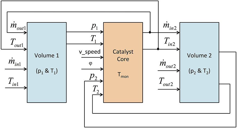 FIGURE 2. Schematic and causality of the catalyst model.
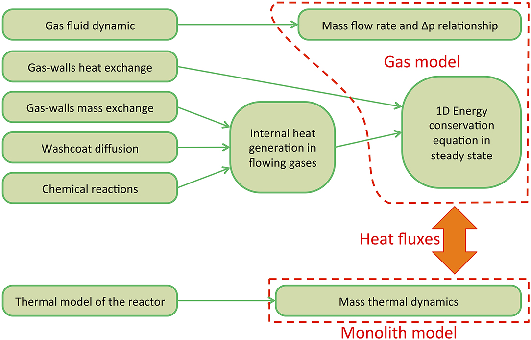 FIGURE 3. Layout of the model of the catalyst core.
The “gas model” has been developed as shown in Figure 4. At each time step values of pressure p and temperature T in the two adjacent volumes are used to calculate pressure difference Δp, mean pressure pm, and temperature Tm (taking account of flow direction). Assuming the catalyst core as a concentrated flow resistance (without mass accumulation) gas mass flow rate can be estimated through an empirical algebraic correlation in the following form:
where ρ and μ (as other fluid properties) are calculated at pm and Tm with regard to the composition of exhaust gases. The geometry of the catalyst involves both the overall dimensions of the core and its morphological characteristics (honeycomb/foam, porosity, etc.). Then gas temperature at the core exit can be defined integrating the energy conservation equation in 1D and in steady state: